MBSStools - an R toolkit for the MBSS program’s data needs
Erik.Leppo@tetratech.com
2022-01-12
Source:vignettes/MBSStools_vignette.Rmd
MBSStools_vignette.RmdIntroduction
MBSStools was created by Tetra Tech, Inc. in 2017 to meet the needs of Maryland Department of Natural Resources (DNR), Maryland Biological Stream Survey (MBSS) staff to complete data manipulations in an efficient and reproducible manner.
It is envisioned that this library will be a living program and will add additional functions and routines in the future.
Many of the examples in this vignette are included in the example sections in the corresponding functions. Each function in the MBSStools library includes example data from MBSS.
Installation
The R library is saved on GitHub (https://github.com/leppott/MBSStools) for ease of updating and distribution. Issues can be tracked, fixed, and code is available for download. Current users of MBSStools can update the library using the same code used to install the library (see below). Devtools is required to download from GitHub. At this time, there are no plans to submit MBSStools to CRAN (R’s library repository).
install.packages("devtools")
library(devtools)
install_github("leppott/MBSStools")
To contact the author directly email Erik.Leppo@tetratech.com.
Packages
Several packages were used to build the functionality in MBSStools.
FlowSum; no extra packages
IonContrib; no extra packages
MapTaxaObs;
readxlandrgdalmetric.scores;
dplyrmetric.values;
dplyrPHIcalc; no extra packages
These packages should install automatically when MBSStools installs. But if you encounter issues with a function not working ensure that the necessary package dependencies are installed.
To install packages follow the example of the code below for installing dplyr.
install.packages("dplyr")Contents
There are several functions included in the library each with a particular focus on a dataset and the necessary calculations for data analysis.
Index of Biological Integrity (IBI) calculations for fish and benthic macroinvertebrates.
Taxonomic distribution maps for fish.
Stream discharge calculation.
Ion contribution to conductivity.
Physical Habitat Index (PHI) calculation.
Example data are included with each function.
IBI
MBSStools calculates both the benthic macroinvertebrate IBI (BIBI) and fish IBI (FIBI). The IBIs are described in the document Southerland et al. 2005 that is included in the /extdata folder of the library.
There are two functions; metric.values() to calculate the metrics (e.g., total individuals or total taxa) and metric.scores() that converts the metric values to the appropriate score (e.g., 1, 3, or 5). The functions are the same for fish and benthic macroinvertebrates. Only the argument fun.Community needs to be changed to “bugs” or “fish”.
MBSStools does not aggregate or compile taxa lists. Taxa data with site/sample information, counts, phylogenetic (phylum, class, order, etc), and autecological (habit, tolerance value, and function feeding group) information is required as an input to the functions. Fish data needs the additional values of watershed (catchment) area (in acres), average stream width, and reach length.
A background table (metrics_scoring) is included and provides a table with the metric names and scoring thresholds for each IBI and index region. This table is populated with the appropriate values for the MBSS IBIs. This table can be modified.
The functions metric.values() and metric.scores() require the dplyr library.
IBI, Fish
Calculates the fish IBI.
The adjustment of metrics based on watershed area is automatic for fish metrics.
Fish metric values assumes the following fields (all upper case)
SITE = MBSS sample identifier.
FIBISTRATA = Fish region (COASTAL, COLD, EPIEDMONT, HIGHLAND).
ACREAGE = Catchment area in acres.
LEN_SAMP = Length of stream sampled; typically 75-meters.
AVWID = Average stream width (meters) for sampled site.
SPECIES = MBSS fish taxa name.
TOTAL = Number of sampled individuals corresponding to specified taxon.
TYPE = Fish group identifier (ALL CAPS); SCULPIN, DARTER, MADTOM, etc.
TROPHIC_MBSS = MBSS tropic status designations (ALL CAPS); OM, GE, IS, IV, etc.
PTOLR = Pollution tolerance level (ALL CAPS); T, I, NO TYPE.
** Sites with a single record indicating “No Fish Observed” receive a default score of 1.00.
# Metrics, Fish
library(MBSStools)
#(generate values then scores)
myIndex <- "MBSS.2005.Fish"
# Thresholds
thresh <- metrics_scoring
# get metric names for myIndex
(myMetrics.Fish <- as.character(droplevels(unique(thresh[thresh[,"Index.Name"]==myIndex,"MetricName.Other"]))))
#>  [1] "ABUNSQM"   "NUMBENTSP" "PTOL"      "PGEOMIV"   "PROUND"    "PABDOM"
#>  [7] "BIOM_MSQ"  "P_LITH"    "P_IS"      "PBROOK"    "PSCULP"
# Taxa Data
myDF.Fish <- taxa_fish
myMetric.Values.Fish <- metric.values(myDF.Fish, "fish", myMetrics.Fish, TRUE)
knitr::kable(head(myMetric.Values.Fish))| Index.Name | SITE | FIBISTRATA | ACREAGE | LEN_SAMP | AVWID | STRMAREA | TOTCNT | ABUNSQM | PABDOM | TOTBIOM | BIOM_MSQ | NUMBENTSP | NUMBROOK | PBROOK | NUMGEOMIV | PGEOMIV | NUMIS | P_IS | NUMLITH | P_LITH | NUMROUND | PROUND | NUMSCULP | PSCULP | NUMTOL | PTOL | NUMBENTSP_Obs | NUMBENTSP_m | NUMBENTSP_b | NUMBENTSP_Exp | NUMBENTSP_Adj |
|---|---|---|---|---|---|---|---|---|---|---|---|---|---|---|---|---|---|---|---|---|---|---|---|---|---|---|---|---|---|---|---|
| MBSS.2005.Fish | _TEST | COASTAL | 10.0000 | 75 | 5.000 | 375.000 | 0 | 0.0000000 | 0.00000 | 0 | 0.000000 | 0.0000000 | 0 | 0 | 0 | 0.00000 | 0 | 0 | 0 | 0.00000 | 0 | 0 | 0 | 0 | 0 | 0.00000 | 0 | 1.69 | -3.33 | -1.6400000 | 0.0000000 |
| MBSS.2005.Fish | CHGX-432-S-1111 | EPIEDMONT | 273.0000 | 75 | 1.500 | 112.500 | 54 | 0.4800000 | 100.00000 | 160 | 1.422222 | 0.0000000 | 0 | 0 | 54 | 100.00000 | 0 | 0 | 0 | 0.00000 | 0 | 0 | 0 | 0 | 54 | 100.00000 | 0 | 1.25 | -2.36 | 0.6852033 | 0.0000000 |
| MBSS.2005.Fish | CHGX-435-R-1111 | EPIEDMONT | 416.1001 | 75 | 3.500 | 262.500 | 539 | 2.0533333 | 71.24304 | 2957 | 11.264762 | 0.0000000 | 0 | 0 | 514 | 95.36178 | 0 | 0 | 155 | 28.75696 | 0 | 0 | 0 | 0 | 514 | 95.36178 | 0 | 1.25 | -2.36 | 0.9139973 | 0.0000000 |
| MBSS.2005.Fish | CHGX-537-R-1111 | EPIEDMONT | 820.6357 | 75 | 2.025 | 151.875 | 104 | 0.6847737 | 60.57692 | 455 | 2.995885 | 0.0000000 | 0 | 0 | 100 | 96.15385 | 0 | 0 | 38 | 36.53846 | 0 | 0 | 0 | 0 | 90 | 86.53846 | 0 | 1.25 | -2.36 | 1.2826880 | 0.0000000 |
| MBSS.2005.Fish | CHGX-546-R-1111 | EPIEDMONT | 1732.0084 | 75 | 3.425 | 256.875 | 139 | 0.5411192 | 40.28777 | 3078 | 11.982482 | 0.5923513 | 0 | 0 | 83 | 59.71223 | 0 | 0 | 76 | 54.67626 | 0 | 0 | 0 | 0 | 60 | 43.16547 | 1 | 1.25 | -2.36 | 1.6881875 | 0.5923513 |
| MBSS.2005.Fish | CHGX-648-S-1111 | EPIEDMONT | 3805.0000 | 75 | 8.950 | 671.250 | 293 | 0.4364991 | 31.39932 | 5020 | 7.478585 | 0.4727142 | 0 | 0 | 201 | 68.60068 | 0 | 0 | 141 | 48.12287 | 0 | 0 | 0 | 0 | 138 | 47.09898 | 1 | 1.25 | -2.36 | 2.1154433 | 0.4727142 |
# SCORE
Metrics.Fish.Scores <- metric.scores(myMetric.Values.Fish
                                     , myMetrics.Fish
                                     , "Index.Name"
                                     , "FIBISTRATA"
                                     , thresh)
#> One or more fish samples (n = 1) had zero organisms and was scored as a 1
#>                               (metrics and IBI).
# View Results
knitr::kable(head(Metrics.Fish.Scores))| Index.Name | SITE | FIBISTRATA | ACREAGE | LEN_SAMP | AVWID | STRMAREA | TOTCNT | ABUNSQM | PABDOM | TOTBIOM | BIOM_MSQ | NUMBENTSP | NUMBROOK | PBROOK | NUMGEOMIV | PGEOMIV | NUMIS | P_IS | NUMLITH | P_LITH | NUMROUND | PROUND | NUMSCULP | PSCULP | NUMTOL | PTOL | NUMBENTSP_Obs | NUMBENTSP_m | NUMBENTSP_b | NUMBENTSP_Exp | NUMBENTSP_Adj | Index.Region | SC_ABUNSQM | SC_NUMBENTSP | SC_PTOL | SC_PGEOMIV | SC_PROUND | SC_PABDOM | SC_BIOM_MSQ | SC_P_LITH | SC_P_IS | SC_PBROOK | SC_PSCULP | sum_IBI | IBI |
|---|---|---|---|---|---|---|---|---|---|---|---|---|---|---|---|---|---|---|---|---|---|---|---|---|---|---|---|---|---|---|---|---|---|---|---|---|---|---|---|---|---|---|---|---|---|
| MBSS.2005.Fish | _TEST | COASTAL | 10.0000 | 75 | 5.000 | 375.000 | 0 | 0.0000000 | 0.00000 | 0 | 0.000000 | 0.0000000 | 0 | 0 | 0 | 0.00000 | 0 | 0 | 0 | 0.00000 | 0 | 0 | 0 | 0 | 0 | 0.00000 | 0 | 1.69 | -3.33 | -1.6400000 | 0.0000000 | COASTAL | 1 | 1 | 1 | 1 | 1 | 1 | 0 | 0 | 0 | 0 | 0 | 6 | 1.000000 |
| MBSS.2005.Fish | CHGX-432-S-1111 | EPIEDMONT | 273.0000 | 75 | 1.500 | 112.500 | 54 | 0.4800000 | 100.00000 | 160 | 1.422222 | 0.0000000 | 0 | 0 | 54 | 100.00000 | 0 | 0 | 0 | 0.00000 | 0 | 0 | 0 | 0 | 54 | 100.00000 | 0 | 1.25 | -2.36 | 0.6852033 | 0.0000000 | EPIEDMONT | 3 | 1 | 1 | 1 | 0 | 0 | 1 | 1 | 0 | 0 | 0 | 8 | 1.333333 |
| MBSS.2005.Fish | CHGX-435-R-1111 | EPIEDMONT | 416.1001 | 75 | 3.500 | 262.500 | 539 | 2.0533333 | 71.24304 | 2957 | 11.264762 | 0.0000000 | 0 | 0 | 514 | 95.36178 | 0 | 0 | 155 | 28.75696 | 0 | 0 | 0 | 0 | 514 | 95.36178 | 0 | 1.25 | -2.36 | 0.9139973 | 0.0000000 | EPIEDMONT | 5 | 1 | 1 | 3 | 0 | 0 | 5 | 1 | 0 | 0 | 0 | 16 | 2.666667 |
| MBSS.2005.Fish | CHGX-537-R-1111 | EPIEDMONT | 820.6357 | 75 | 2.025 | 151.875 | 104 | 0.6847737 | 60.57692 | 455 | 2.995885 | 0.0000000 | 0 | 0 | 100 | 96.15385 | 0 | 0 | 38 | 36.53846 | 0 | 0 | 0 | 0 | 90 | 86.53846 | 0 | 1.25 | -2.36 | 1.2826880 | 0.0000000 | EPIEDMONT | 3 | 1 | 1 | 3 | 0 | 0 | 1 | 3 | 0 | 0 | 0 | 12 | 2.000000 |
| MBSS.2005.Fish | CHGX-546-R-1111 | EPIEDMONT | 1732.0084 | 75 | 3.425 | 256.875 | 139 | 0.5411192 | 40.28777 | 3078 | 11.982482 | 0.5923513 | 0 | 0 | 83 | 59.71223 | 0 | 0 | 76 | 54.67626 | 0 | 0 | 0 | 0 | 60 | 43.16547 | 1 | 1.25 | -2.36 | 1.6881875 | 0.5923513 | EPIEDMONT | 3 | 5 | 5 | 5 | 0 | 0 | 5 | 3 | 0 | 0 | 0 | 26 | 4.333333 |
| MBSS.2005.Fish | CHGX-648-S-1111 | EPIEDMONT | 3805.0000 | 75 | 8.950 | 671.250 | 293 | 0.4364991 | 31.39932 | 5020 | 7.478585 | 0.4727142 | 0 | 0 | 201 | 68.60068 | 0 | 0 | 141 | 48.12287 | 0 | 0 | 0 | 0 | 138 | 47.09898 | 1 | 1.25 | -2.36 | 2.1154433 | 0.4727142 | EPIEDMONT | 3 | 5 | 3 | 5 | 0 | 0 | 3 | 3 | 0 | 0 | 0 | 22 | 3.666667 |
#Write results to csv file
#write.csv(Metrics.Fish.Scores, "Filename.csv")
IBI, Benthic Macroinvertebrates, MBSS
Bug metric values assumes the following fields (all upper case)
SITE = MBSS sample identifier.
TAXON = MBSS benthic macroinvertebrate name.
N_TAXA = Number of sampled individuals corresponding to specified taxon.
EXCLUDE = Non-unique taxa (i.e., parent taxon with one or more children taxa present in sample). “Y” = do not include in taxa richness metrics.
STRATA_R = Benthic macroinvertebrate region (COASTAL, EPIEDMONT, or HIGHLAND).
Phylogenetic fields:
PHYLUM, CLASS, ORDER, FAMILY, GENUS, OTHER_TAXA, TRIBE
Autoecological fields:
FFG, HABIT, FINALTOLVAL07
Valid values for FFG: COLLECTOR, FILTERER, PIERCER, PREDATOR, SCRAPER, SHREDDER
Valid values for HABIT: BU, CB, CN, SP, SW
Maryland Stream Waders (MSW) data should be first combined to family level and EXCLUDE recalculated.
Additional fields needed:
- FAM_TV (need to include all the same fields, just leave blank).
In addition to the metric scores a QC check on samples with too many (>120) or too few (<60) organisms is returned in the results. Those with more than the maximum (120) should be subsampled down to within the target range.
# Metrics, Index, Benthic Macroinvertebrates, genus
# (generate values then scores)
myIndex <- "MBSS.2005.Bugs"
# Thresholds
thresh <- metrics_scoring
# get metric names for myIndex
(myMetrics.Bugs.MBSS <- as.character(droplevels(unique(thresh[thresh[,"Index.Name"]==myIndex,"MetricName.Other"]))))
#>  [1] "ntaxa"      "nept"       "nephem"     "pintol_urb" "pephem"
#>  [6] "nscrape"    "pclimb"     "pchiron"    "pcling"     "ptany"
#> [11] "pscrape"    "pswim"      "pdipt"
# Taxa Data
myDF.Bugs.MBSS <- taxa_bugs_genus
myMetric.Values.Bugs.MBSS <- metric.values(myDF.Bugs.MBSS, "bugs", myMetrics.Bugs.MBSS)
# SCORE
Metrics.Bugs.Scores.MBSS <- metric.scores(myMetric.Values.Bugs.MBSS, myMetrics.Bugs.MBSS, "INDEX.NAME", "STRATA_R", thresh)
#> One or more bug samples had < 60 (n = 0) or > 120 (n = 90) organisms.
#>
#>                                  These samples should be further examined.
#Write results to csv file
#write.csv(Metrics.Bugs.Scores.MBSS, "Filename.csv")

# QC bug count
Metrics.Bugs.Scores.MBSS[Metrics.Bugs.Scores.MBSS[,"totind"]>120,"QC_Count"] <- "LARGE"
Metrics.Bugs.Scores.MBSS[Metrics.Bugs.Scores.MBSS[,"totind"]<60,"QC_Count"] <- "SMALL"
Metrics.Bugs.Scores.MBSS[is.na(Metrics.Bugs.Scores.MBSS[,"QC_Count"]),"QC_Count"] <- "OK"
# table of QC_Count
knitr::kable(head(Metrics.Bugs.Scores.MBSS))| SITE | STRATA_R | INDEX.NAME | totind | ntaxa | nept | nephem | totephem | nscrape | totclimb | totchiron | totcling | tottany | totscrape | totswim | totdipt | totintol_urb | pephem | pclimb | pchiron | pcling | ptany | pscrape | pswim | pdipt | pintol_urb | ndipt | nintol | becks | nintol_FAM | Index.Name | Index.Region | SC_ntaxa | SC_nept | SC_nephem | SC_pintol_urb | SC_pephem | SC_nscrape | SC_pclimb | SC_pchiron | SC_pcling | SC_ptany | SC_pscrape | SC_pswim | SC_pdipt | sum_IBI | IBI | QC_Count |
|---|---|---|---|---|---|---|---|---|---|---|---|---|---|---|---|---|---|---|---|---|---|---|---|---|---|---|---|---|---|---|---|---|---|---|---|---|---|---|---|---|---|---|---|---|---|---|---|
| CHGX-432-S-1111 | EPIEDMONT | MBSS.2005.Bugs | 125 | 27 | 10 | 1 | 13 | 4 | 31 | 50 | 82 | 2 | 9 | 13 | 57 | 45 | 10.400000 | 24.800000 | 40.00000 | 65.60000 | 1.600000 | 7.200000 | 10.400000 | 45.60000 | 36.00000 | 11 | 10 | 18 | 6 | MBSS.2005.Bugs | EPIEDMONT | 5 | 3 | 1 | 3 | 0 | 0 | 0 | 3 | 3 | 0 | 0 | 0 | 0 | 18 | 3.000000 | LARGE |
| CHGX-435-R-1111 | EPIEDMONT | MBSS.2005.Bugs | 119 | 17 | 2 | 0 | 0 | 1 | 9 | 81 | 39 | 2 | 3 | 0 | 85 | 0 | 0.000000 | 7.563025 | 68.06723 | 32.77311 | 1.680672 | 2.521008 | 0.000000 | 71.42857 | 0.00000 | 11 | 0 | 0 | 0 | MBSS.2005.Bugs | EPIEDMONT | 3 | 1 | 1 | 1 | 0 | 0 | 0 | 1 | 3 | 0 | 0 | 0 | 0 | 10 | 1.666667 | OK |
| CHGX-537-R-1111 | EPIEDMONT | MBSS.2005.Bugs | 121 | 29 | 10 | 4 | 12 | 6 | 18 | 40 | 82 | 12 | 12 | 11 | 50 | 16 | 9.917355 | 14.876033 | 33.05785 | 67.76860 | 9.917355 | 9.917355 | 9.090909 | 41.32231 | 13.22314 | 11 | 8 | 14 | 5 | MBSS.2005.Bugs | EPIEDMONT | 5 | 3 | 5 | 3 | 0 | 0 | 0 | 3 | 3 | 0 | 0 | 0 | 0 | 22 | 3.666667 | LARGE |
| CHGX-546-R-1111 | EPIEDMONT | MBSS.2005.Bugs | 129 | 27 | 8 | 2 | 23 | 4 | 22 | 28 | 97 | 0 | 11 | 23 | 37 | 14 | 17.829457 | 17.054264 | 21.70543 | 75.19380 | 0.000000 | 8.527132 | 17.829457 | 28.68217 | 10.85271 | 11 | 7 | 15 | 7 | MBSS.2005.Bugs | EPIEDMONT | 5 | 3 | 3 | 1 | 0 | 0 | 0 | 5 | 5 | 0 | 0 | 0 | 0 | 22 | 3.666667 | LARGE |
| CHGX-648-S-1111 | EPIEDMONT | MBSS.2005.Bugs | 116 | 27 | 13 | 4 | 40 | 6 | 32 | 31 | 80 | 2 | 14 | 35 | 38 | 26 | 34.482759 | 27.586207 | 26.72414 | 68.96552 | 1.724138 | 12.068965 | 30.172414 | 32.75862 | 22.41379 | 10 | 12 | 20 | 8 | MBSS.2005.Bugs | EPIEDMONT | 5 | 5 | 5 | 3 | 0 | 0 | 0 | 3 | 3 | 0 | 0 | 0 | 0 | 24 | 4.000000 | OK |
| EBUX-435-S-1111 | EPIEDMONT | MBSS.2005.Bugs | 137 | 37 | 15 | 5 | 40 | 5 | 15 | 34 | 98 | 12 | 13 | 39 | 46 | 78 | 29.197080 | 10.948905 | 24.81752 | 71.53285 | 8.759124 | 9.489051 | 28.467153 | 33.57664 | 56.93431 | 16 | 19 | 38 | 10 | MBSS.2005.Bugs | EPIEDMONT | 5 | 5 | 5 | 5 | 0 | 0 | 0 | 3 | 3 | 0 | 0 | 0 | 0 | 26 | 4.333333 | LARGE |
IBI, Benthic Macroinvertebrates, MSW
The Maryland Stream Wader index is from Stribling et al. 1999. Metric values and scores shown below for example data.
SITE = Sample identifier.
TAXON = MSW benthic macroinvertebrate name (Family-level identification).
N_TAXA = Number of taxon collected in sample.
EXCLUDE = Non-unique taxa (i.e., parent taxon with one or more children taxa present in sample).
“Y” = do not include in taxa richness metrics.
STRATA_R =This index has only two bioregions (CP=Coastal Plain, NCP=Non-Coastal Plain).
Phylogenetic fields:
PHYLUM, CLASS, ORDER, FAMILY
Autoecological field:
FAM_TV
# Metrics, MSW Index, Benthic Macroinvertebrates, family
myIndex <- "MSW.1999.Bugs"
# Thresholds
thresh <- metrics_scoring
# get metric names for myIndex
(myMetrics.Bugs.MSW <- as.character(droplevels(unique(thresh[thresh[,"Index.Name"]==myIndex,"MetricName.Other"]))))
#> [1] "ntaxa"      "nept"       "nephem"     "ndipt"      "pephem"
#> [6] "nintol_FAM" "becks"
# Taxa Data
myDF.Bugs.MSW <- taxa_bugs_family
myMetric.Values.Bugs.MSW <- metric.values(myDF.Bugs.MSW, "bugs", myMetrics.Bugs.MSW)
knitr::kable(head(myMetric.Values.Bugs.MSW))| SITE | STRATA_R | INDEX.NAME | totind | ntaxa | nept | nephem | totephem | nscrape | totclimb | totchiron | totcling | tottany | totscrape | totswim | totdipt | totintol_urb | pephem | pclimb | pchiron | pcling | ptany | pscrape | pswim | pdipt | pintol_urb | ndipt | nintol | becks | nintol_FAM |
|---|---|---|---|---|---|---|---|---|---|---|---|---|---|---|---|---|---|---|---|---|---|---|---|---|---|---|---|---|---|
| CHGX-432-S-1111 | NCP | MSW.1999.Bugs | 125 | 16 | 7 | 1 | 13 | 0 | 0 | 50 | 0 | 0 | 0 | 0 | 57 | 0 | 10.400000 | 0 | 40.00000 | 0 | 0 | 0 | 0 | 45.60000 | 0 | 3 | 1 | 3 | 5 |
| CHGX-435-R-1111 | NCP | MSW.1999.Bugs | 119 | 7 | 1 | 0 | 0 | 0 | 0 | 81 | 0 | 0 | 0 | 0 | 85 | 0 | 0.000000 | 0 | 68.06723 | 0 | 0 | 0 | 0 | 71.42857 | 0 | 3 | 1 | 3 | 0 |
| CHGX-537-R-1111 | NCP | MSW.1999.Bugs | 121 | 18 | 8 | 3 | 12 | 0 | 0 | 40 | 0 | 0 | 0 | 0 | 50 | 0 | 9.917355 | 0 | 33.05785 | 0 | 0 | 0 | 0 | 41.32231 | 0 | 3 | 1 | 3 | 5 |
| CHGX-546-R-1111 | NCP | MSW.1999.Bugs | 129 | 17 | 6 | 2 | 23 | 0 | 0 | 28 | 0 | 0 | 0 | 0 | 37 | 0 | 17.829457 | 0 | 21.70543 | 0 | 0 | 0 | 0 | 28.68217 | 0 | 4 | 1 | 3 | 6 |
| CHGX-648-S-1111 | NCP | MSW.1999.Bugs | 116 | 18 | 11 | 4 | 40 | 0 | 0 | 31 | 0 | 0 | 0 | 0 | 38 | 0 | 34.482759 | 0 | 26.72414 | 0 | 0 | 0 | 0 | 32.75862 | 0 | 3 | 1 | 3 | 8 |
| EBUX-435-S-1111 | NCP | MSW.1999.Bugs | 137 | 19 | 10 | 3 | 40 | 0 | 0 | 34 | 0 | 0 | 0 | 0 | 46 | 0 | 29.197080 | 0 | 24.81752 | 0 | 0 | 0 | 0 | 33.57664 | 0 | 4 | 1 | 3 | 9 |
# SCORE
Metrics.Bugs.Scores.MSW <- metric.scores(myMetric.Values.Bugs.MSW, myMetrics.Bugs.MSW, "INDEX.NAME", "STRATA_R", thresh)
#> One or more bug samples had < 60 (n = 0) or > 120 (n = 102) organisms.
#>
#>                                  These samples should be further examined.
# View Results
knitr::kable(head(Metrics.Bugs.Scores.MSW))| SITE | STRATA_R | INDEX.NAME | totind | ntaxa | nept | nephem | totephem | nscrape | totclimb | totchiron | totcling | tottany | totscrape | totswim | totdipt | totintol_urb | pephem | pclimb | pchiron | pcling | ptany | pscrape | pswim | pdipt | pintol_urb | ndipt | nintol | becks | nintol_FAM | Index.Name | Index.Region | SC_ntaxa | SC_nept | SC_nephem | SC_ndipt | SC_pephem | SC_nintol_FAM | SC_becks | sum_IBI | IBI |
|---|---|---|---|---|---|---|---|---|---|---|---|---|---|---|---|---|---|---|---|---|---|---|---|---|---|---|---|---|---|---|---|---|---|---|---|---|---|---|---|---|
| CHGX-432-S-1111 | NCP | MSW.1999.Bugs | 125 | 16 | 7 | 1 | 13 | 0 | 0 | 50 | 0 | 0 | 0 | 0 | 57 | 0 | 10.400000 | 0 | 40.00000 | 0 | 0 | 0 | 0 | 45.60000 | 0 | 3 | 1 | 3 | 5 | MSW.1999.Bugs | NCP | 5 | 3 | 1 | 5 | 3 | 3 | 1 | 21 | 3.000000 |
| CHGX-435-R-1111 | NCP | MSW.1999.Bugs | 119 | 7 | 1 | 0 | 0 | 0 | 0 | 81 | 0 | 0 | 0 | 0 | 85 | 0 | 0.000000 | 0 | 68.06723 | 0 | 0 | 0 | 0 | 71.42857 | 0 | 3 | 1 | 3 | 0 | MSW.1999.Bugs | NCP | 1 | 1 | 1 | 5 | 1 | 1 | 1 | 11 | 1.571429 |
| CHGX-537-R-1111 | NCP | MSW.1999.Bugs | 121 | 18 | 8 | 3 | 12 | 0 | 0 | 40 | 0 | 0 | 0 | 0 | 50 | 0 | 9.917355 | 0 | 33.05785 | 0 | 0 | 0 | 0 | 41.32231 | 0 | 3 | 1 | 3 | 5 | MSW.1999.Bugs | NCP | 5 | 3 | 5 | 5 | 3 | 3 | 1 | 25 | 3.571429 |
| CHGX-546-R-1111 | NCP | MSW.1999.Bugs | 129 | 17 | 6 | 2 | 23 | 0 | 0 | 28 | 0 | 0 | 0 | 0 | 37 | 0 | 17.829457 | 0 | 21.70543 | 0 | 0 | 0 | 0 | 28.68217 | 0 | 4 | 1 | 3 | 6 | MSW.1999.Bugs | NCP | 5 | 3 | 3 | 5 | 3 | 3 | 1 | 23 | 3.285714 |
| CHGX-648-S-1111 | NCP | MSW.1999.Bugs | 116 | 18 | 11 | 4 | 40 | 0 | 0 | 31 | 0 | 0 | 0 | 0 | 38 | 0 | 34.482759 | 0 | 26.72414 | 0 | 0 | 0 | 0 | 32.75862 | 0 | 3 | 1 | 3 | 8 | MSW.1999.Bugs | NCP | 5 | 5 | 5 | 5 | 5 | 5 | 1 | 31 | 4.428571 |
| EBUX-435-S-1111 | NCP | MSW.1999.Bugs | 137 | 19 | 10 | 3 | 40 | 0 | 0 | 34 | 0 | 0 | 0 | 0 | 46 | 0 | 29.197080 | 0 | 24.81752 | 0 | 0 | 0 | 0 | 33.57664 | 0 | 4 | 1 | 3 | 9 | MSW.1999.Bugs | NCP | 5 | 5 | 5 | 5 | 5 | 5 | 1 | 31 | 4.428571 |
Fish Distribution Maps
The intent of this function is to recreate the taxa distribution maps on the MBSS website: http://eyesonthebay.dnr.maryland.gov/mbss/fishes.cfm. The maps for all taxa can be generated from a single line of code. The maps generated with this function use a ‘crosswalk’ table that converts taxa names to map names.
The function MapTaxaObs() requires the readxl and rgdal packages.
Data inputs
The user will need GIS files for the state of Maryland for State, County, and Water.
The inputs for this function, besides the three GIS shapefiles, are taxa observations and a taxa name crosswalk (translation) table between taxa names and map names.
All inputs are included in the MBSStools library and can be copied to the current directory with the code below.
# Set Working Directory
wd <- getwd()
# Create Example Data if Needed
## Create Directories
myDir.create <- file.path(wd,"Data")
ifelse(dir.exists(myDir.create)==FALSE,dir.create(myDir.create),"Directory already exists")
myDir.create <- file.path(wd,"GIS")
ifelse(dir.exists(myDir.create)==FALSE,dir.create(myDir.create),"Directory already exists")
myDir.create <- file.path(wd,"Maps")
ifelse(dir.exists(myDir.create)==FALSE,dir.create(myDir.create),"Directory already exists")
## Create Data
### Taxa Data
myFiles <- c("AllFish_95to16.xls", "TaxaMapsCrossWalk20170731.xlsx")
file.copy(file.path(path.package("MBSStools"),"extdata",myFiles),file.path(wd,"Data",myFiles))
### GIS
unzip(file.path(path.package("MBSStools"),"extdata","MD_GIS.zip"),exdir=file.path(wd,"GIS"))
Example Input Data
Observation data with three columns needed for the tool to work (common name, latitude, and longitude). Additional columns can be appended (e.g., SiteYr) and will not affect the functionality.
#>             CommonName Latitude83 Longitude83
#> 1    eastern mudminnow     39.055   -76.73417
#> 2           creek chub     39.055   -76.73417
#> 3      channel catfish     39.055   -76.73417
#> 4        glassy darter     39.055   -76.73417
#> 5 eastern mosquitofish     39.055   -76.73417
#> 6        golden shiner     39.055   -76.73417
Crosswalk data with common name and map name.
#>         CommonName  MapName
#> 1          alewife  alewife
#> 2     american eel  amereel
#> 3    american shad amershad
#> 4    banded darter bandartr
#> 5 banded killifish bankilli
#> 6    black crappie blkcrapi
Map Creation
The code below can be used to generate the maps (n=131) associated with the 1995 to 2016 data. Any taxa without a match in the crosswalk table (n=54) are listed in a CSV file and the number reported to the user in the R console, but maps are not generated (by default). If the user wants all maps then the parameter ‘onlymatches’ should be set to ‘FALSE’ (as in the example below).
# Set Working Directory
wd <- getwd()

# Inputs
Obs <- "AllFish_95to16.xls"
XWalk <- "TaxaMapsCrossWalk20170731.xlsx"
wd <- getwd()

# Create maps
MapTaxaObs(Obs, XWalk, wd, onlymatches = FALSE)
The intent behind this function was to recreate the fish taxa distribution maps. But the data inputs are not specific to fish and can be used for benthic macroinvertebrate data.
The taxa distribution map for brown trout is shown below.
#> Loading required package: sp
#> Please note that rgdal will be retired by the end of 2023,
#> plan transition to sf/stars/terra functions using GDAL and PROJ
#> at your earliest convenience.
#>
#> rgdal: version: 1.5-28, (SVN revision 1158)
#> Geospatial Data Abstraction Library extensions to R successfully loaded
#> Loaded GDAL runtime: GDAL 3.2.1, released 2020/12/29
#> Path to GDAL shared files: /Users/runner/work/_temp/Library/rgdal/gdal
#> GDAL binary built with GEOS: TRUE
#> Loaded PROJ runtime: Rel. 7.2.1, January 1st, 2021, [PJ_VERSION: 721]
#> Path to PROJ shared files: /Users/runner/work/_temp/Library/rgdal/proj
#> PROJ CDN enabled: FALSE
#> Linking to sp version:1.4-6
#> To mute warnings of possible GDAL/OSR exportToProj4() degradation,
#> use options("rgdal_show_exportToProj4_warnings"="none") before loading sp or rgdal.
#> Overwritten PROJ_LIB was /Users/runner/work/_temp/Library/rgdal/proj
#> Linking to GEOS 3.8.1, GDAL 3.2.1, PROJ 7.2.1; sf_use_s2() is TRUE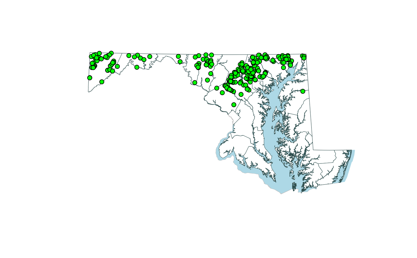
Stream Discharge
Calculate stream discharge based on field measurements. Side channels that are properly identified in the data will be included.
The function FlowSum() requires no additional packages.
library(MBSStools)
# data
MBSS.flow <- MBSS.flow
# calculate flow
flow.cell <- FlowSum(MBSS.flow, returnType="cell")
flow.sample <- FlowSum(MBSS.flow)
# examine data
View(flow.cell)
View(flow.sample)
# Example Save file (tab delimited text file)
datetime <- format(Sys.time(),"%Y%m%d_%H%M%S")
myYear <- "15"
#write.table(flow.sample,paste0("SumFlow",myYear,"_",datetime,".tab"),row.names=FALSE,sep="\t")
Ion Matrix
The IonContrib() function calculates conductivity contribution from provided ion concentrations using Kohlrausch’s Law. If a total conductivity measurement is not provided, the total conductivity is calculated as the sum of all ions present in the data. If the user provides a conductivity measurement, then ion contributions are a percentage of that number. In the latter case, “Other” is added as an ion to capture any percentage of total conductivity not represented by the provided ions. Plotting is done outside of this function.
Data will need to be in “wide” format. That is, a single record for each sample and the ions to be analyzed in columns.
A reference table of ions and their equivalent ionic conductance at infinite dilution is provided with the function as “MBSS.Ion.Ref”. The function allows for input of a user supplied data frame if this table needs updating with more ions.
The function IonContrib() requires no additional packages.
| Name | Ion | Symbol | Molecular Weight (g/mole) | Valance | Equivalent Ionic conductance at infinite dilution (µS/cm) | Multiplier | SortOrder |
|---|---|---|---|---|---|---|---|
| Calcium (mg/L) | Calcium | Ca2+ | 40.07800 | 2 | 59.47 | 2.9677130 | 1 |
| Magnesium (mg/L) | Magnesium | Mg2+ | 24.30500 | 2 | 53.00 | 4.3612425 | 2 |
| Sodium (mg/L) | Sodium | Na+ | 22.98977 | 1 | 50.08 | 2.1783604 | 3 |
| Potassium (mg/L) | Potassium | K+ | 39.09830 | 1 | 73.48 | 1.8793656 | 4 |
| Bicarbonate (mg/L) | Bicarbonate | HCO3- | 61.01714 | 1 | 44.50 | 0.7293033 | 5 |
| Sulfate (mg/L) | Sulfate | SO42- | 96.06360 | 2 | 80.00 | 1.6655632 | 6 |
| Chloride (mg/L) | Chloride | Cl- | 35.45270 | 1 | 76.31 | 2.1524454 | 7 |
| Iron (II) (mg/L) | Iron (II) | Fe2+ | 55.84700 | 2 | 54.00 | 1.9338550 | 8 |
| Iron (III) (mg/L) | Iron (III) | Fe3+ | 55.84700 | 3 | 68.00 | 3.6528372 | 9 |
| Bromide (mg/L) | Bromide | Br- | 79.90400 | 1 | 78.10 | 0.9774229 | 10 |
| Strontium (mg/L) | Strontium | Sr2+ | 87.62000 | 2 | 59.40 | 1.3558548 | 11 |
| Nitrate-N (mg/L) | Nitrate-N | NO3- | 14.00674 | 1 | 71.42 | 5.0989738 | 12 |
| Barium (mg/L) | Barium | Ba2+ | 137.32700 | 2 | 63.60 | 0.9262563 | 13 |
The columns for the ions need to match the reference table names. The function IonContrib() includes a reference table that is used by default but the user can supply their own reference table.
| Site | Stream Name | SHA Road Crossing | Ion Matrix | Date Collected | Time Collected | Chloride (mg/L) | Bromide (mg/L) | Nitrate-N (mg/L) | Sulfate (mg/L) | Sodium (mg/L) | Potassium (mg/L) | Magnesium (mg/L) | Calcium (mg/L) |
|---|---|---|---|---|---|---|---|---|---|---|---|---|---|
| BELK-101-X | Gramies Run | MD 273 (Telegraph Rd.) | Pre-Application Baseline | 2016-12-14 | 1899-12-30 10:48:00 | 40.9854 | 0.0255 | 0.6209 | 11.2139 | 19.36 | 1.897 | 8.153 | 12.11 |
| BELK-102-X | Gramies Run | MD 273 (Telegraph Rd.) | Pre-Application Baseline | 2016-12-14 | 1899-12-30 10:59:00 | 36.2214 | 0.0244 | 0.5236 | 13.5295 | 16.08 | 2.103 | 9.403 | 14.09 |
| BELK-301-X | Big Elk Creek | MD 273 (Telegraph Rd.) | Pre-Application Baseline | 2016-12-14 | 1899-12-30 09:15:00 | 31.3782 | 0.0276 | 4.8693 | 13.5987 | 14.06 | 3.166 | 6.906 | 15.73 |
| BELK-302-X | Big Elk Creek | MD 273 (Telegraph Rd.) | Pre-Application Baseline | 2016-12-14 | 1899-12-30 09:19:00 | 30.4018 | 0.0280 | 4.5474 | 13.7224 | 14.01 | 3.049 | 6.583 | 15.92 |
| BRIG-301-X | Patuxent River | MD 94 (Woodbine Rd.) | Pre-Application Baseline | 2016-12-13 | 1899-12-30 14:53:00 | 37.2093 | 0.0232 | 3.0927 | 4.2891 | 19.02 | 2.020 | 5.977 | 10.99 |
| BRIG-302-X | Patuxent River | MD 94 (Woodbine Rd.) | Pre-Application Baseline | 2016-12-13 | 1899-12-30 15:02:00 | 37.6789 | 0.0215 | 3.0869 | 4.2854 | 18.62 | 2.035 | 5.958 | 11.00 |
Example code is below. The user would then save the output (e.g., write.csv()).
library(MBSStools)
# Load Data
# MBSS.Ion.Data = example dataset
data.ion <- MBSS.Ion.Data
# Load Reference Table
ref.ion <- MBSS.Ion.Ref
# Calculate Percent Contribution by Ion (data table only)
contrib.ion <- IonContrib(data.ion)
No conductivity values provided.
    Ion contributions calculated from the sum of calculated ion conductivity
values.| Site | Stream Name | SHA Road Crossing | Ion Matrix | Date Collected | Time Collected | Chloride (mg/L) | Bromide (mg/L) | Nitrate-N (mg/L) | Sulfate (mg/L) | Sodium (mg/L) | Potassium (mg/L) | Magnesium (mg/L) | Calcium (mg/L) | Mult.Calcium (mg/L) | Mult.Magnesium (mg/L) | Mult.Sodium (mg/L) | Mult.Potassium (mg/L) | Mult.Sulfate (mg/L) | Mult.Chloride (mg/L) | Mult.Bromide (mg/L) | Mult.Nitrate-N (mg/L) | Cond.Calcium (mg/L) | Cond.Magnesium (mg/L) | Cond.Sodium (mg/L) | Cond.Potassium (mg/L) | Cond.Sulfate (mg/L) | Cond.Chloride (mg/L) | Cond.Bromide (mg/L) | Cond.Nitrate-N (mg/L) | Cond.SubTotal | Cond.Total | Cond.Other (mg/L) | PctContrib.Calcium (mg/L) | PctContrib.Magnesium (mg/L) | PctContrib.Sodium (mg/L) | PctContrib.Potassium (mg/L) | PctContrib.Sulfate (mg/L) | PctContrib.Chloride (mg/L) | PctContrib.Bromide (mg/L) | PctContrib.Nitrate-N (mg/L) | PctContrib.Other (mg/L) | QC.PctContrib |
|---|---|---|---|---|---|---|---|---|---|---|---|---|---|---|---|---|---|---|---|---|---|---|---|---|---|---|---|---|---|---|---|---|---|---|---|---|---|---|---|---|---|---|
| BELK-101-X | Gramies Run | MD 273 (Telegraph Rd.) | Pre-Application Baseline | 2016-12-14 | 1899-12-30 10:48:00 | 40.9854 | 0.0255 | 0.6209 | 11.2139 | 19.36 | 1.897 | 8.153 | 12.11 | 2.967713 | 4.3612425 | 2.1783604 | 1.8793656 | 1.6655632 | 2.1524454 | 0.9774229 | 5.098974 | 35.93900 | 35.557210 | 42.17306 | 3.565157 | 18.67746 | 88.21883 | 0.0249243 | 3.165953 | 227.3216 | 227.3216 | 0 | 0.1580976 | 0.1564181 | 0.1855216 | 0.0156833 | 0.0821632 | 0.3880794 | 0.0001096 | 0.0139272 | 0 | 1 |
| BELK-102-X | Gramies Run | MD 273 (Telegraph Rd.) | Pre-Application Baseline | 2016-12-14 | 1899-12-30 10:59:00 | 36.2214 | 0.0244 | 0.5236 | 13.5295 | 16.08 | 2.103 | 9.403 | 14.09 | 4.361243 | 2.1783604 | 1.8793656 | 1.6655632 | 2.1524454 | 0.9774229 | 5.0989738 | 2.967713 | 61.44991 | 20.483123 | 30.22020 | 3.502680 | 29.12151 | 35.40363 | 0.1244150 | 1.553894 | 181.8594 | 181.8594 | 0 | 0.3378980 | 0.1126317 | 0.1661735 | 0.0192604 | 0.1601320 | 0.1946759 | 0.0006841 | 0.0085445 | 0 | 1 |
| BELK-301-X | Big Elk Creek | MD 273 (Telegraph Rd.) | Pre-Application Baseline | 2016-12-14 | 1899-12-30 09:15:00 | 31.3782 | 0.0276 | 4.8693 | 13.5987 | 14.06 | 3.166 | 6.906 | 15.73 | 2.178360 | 1.8793656 | 1.6655632 | 2.1524454 | 0.9774229 | 5.0989738 | 2.9677130 | 4.361243 | 34.26561 | 12.978899 | 23.41782 | 6.814642 | 13.29168 | 159.99662 | 0.0819089 | 21.236198 | 272.0834 | 272.0834 | 0 | 0.1259379 | 0.0477019 | 0.0860685 | 0.0250462 | 0.0488515 | 0.5880426 | 0.0003010 | 0.0780503 | 0 | 1 |
| BELK-302-X | Big Elk Creek | MD 273 (Telegraph Rd.) | Pre-Application Baseline | 2016-12-14 | 1899-12-30 09:19:00 | 30.4018 | 0.0280 | 4.5474 | 13.7224 | 14.01 | 3.049 | 6.583 | 15.92 | 1.879366 | 1.6655632 | 2.1524454 | 0.9774229 | 5.0989738 | 2.9677130 | 4.3612425 | 2.178360 | 29.91950 | 10.964403 | 30.15576 | 2.980162 | 69.97016 | 90.22382 | 0.1221148 | 9.905876 | 244.2418 | 244.2418 | 0 | 0.1224995 | 0.0448916 | 0.1234668 | 0.0122017 | 0.2864791 | 0.3694037 | 0.0005000 | 0.0405577 | 0 | 1 |
| BRIG-301-X | Patuxent River | MD 94 (Woodbine Rd.) | Pre-Application Baseline | 2016-12-13 | 1899-12-30 14:53:00 | 37.2093 | 0.0232 | 3.0927 | 4.2891 | 19.02 | 2.020 | 5.977 | 10.99 | 1.665563 | 2.1524454 | 0.9774229 | 5.0989738 | 2.9677130 | 4.3612425 | 2.1783604 | 1.879366 | 18.30454 | 12.865166 | 18.59058 | 10.299927 | 12.72882 | 162.27878 | 0.0505380 | 5.812314 | 240.9307 | 240.9307 | 0 | 0.0759743 | 0.0533978 | 0.0771615 | 0.0427506 | 0.0528319 | 0.6735497 | 0.0002098 | 0.0241244 | 0 | 1 |
| BRIG-302-X | Patuxent River | MD 94 (Woodbine Rd.) | Pre-Application Baseline | 2016-12-13 | 1899-12-30 15:02:00 | 37.6789 | 0.0215 | 3.0869 | 4.2854 | 18.62 | 2.035 | 5.958 | 11.00 | 2.152445 | 0.9774229 | 5.0989738 | 2.9677130 | 4.3612425 | 2.1783604 | 1.8793656 | 1.665563 | 23.67690 | 5.823486 | 94.94289 | 6.039296 | 18.68967 | 82.07822 | 0.0404064 | 5.141427 | 236.4323 | 236.4323 | 0 | 0.1001424 | 0.0246307 | 0.4015648 | 0.0255434 | 0.0790487 | 0.3471532 | 0.0001709 | 0.0217459 | 0 | 1 |
Dot charts are a good way to display the data. But any chart of the user’s preference can be used.
# Load Data
data.ion <- MBSS.Ion.Data
# Load Reference Table
ref.ion <- MBSS.Ion.Ref
# Calculate Percent Contribution by Ion (data table only)
contrib.ion <- IonContrib(data.ion)
knitr::kable(contrib.ion)
# Calculate Percent Contribution by Ion (data table and reference table)
contrib.ion.2 <- IonContrib(data.ion, ref.ion)
knitr::kable(contrib.ion.2)
# Calculate Percent Contribution by Ion (data table, reference table, and conductivity values)
# ## add dummy conductivity values for each sample
myCond <- "Cond"
data.ion[,myCond] <- 4000
contrib.ion.3 <- IonContrib(data.ion, ref.ion, myCond)
knitr::kable(contrib.ion.3)
# Save Results (use write.table())
# Plot Results
myIons <- c("Chloride (mg/L)", "Bromide (mg/L)", "Nitrate-N (mg/L)", "Sulfate (mg/L)", "Sodium (mg/L)",
"Potassium (mg/L)", "Magnesium (mg/L)", "Calcium (mg/L)" )
myIons.Contrib <- paste0("PctContrib.",myIons)
mySite <- "BELK-101-X"
data.plot <- subset(contrib.ion, contrib.ion[,"Site"]==mySite, select=c("Site","Cond.Total",myIons.Contrib,myIons))
## Plot, one site (with cond value)
dotchart(as.numeric(as.vector(data.plot[,myIons.Contrib])), labels=myIons, main=mySite, xlab="Percent Contribution", pch=19, pt.cex=1.2)
mtext(paste0("Conductivity (uS/cm) = ",round(data.plot[,"Cond.Total"],1)))
## Plot all sites using panel.dotplot() in the lattice package
#
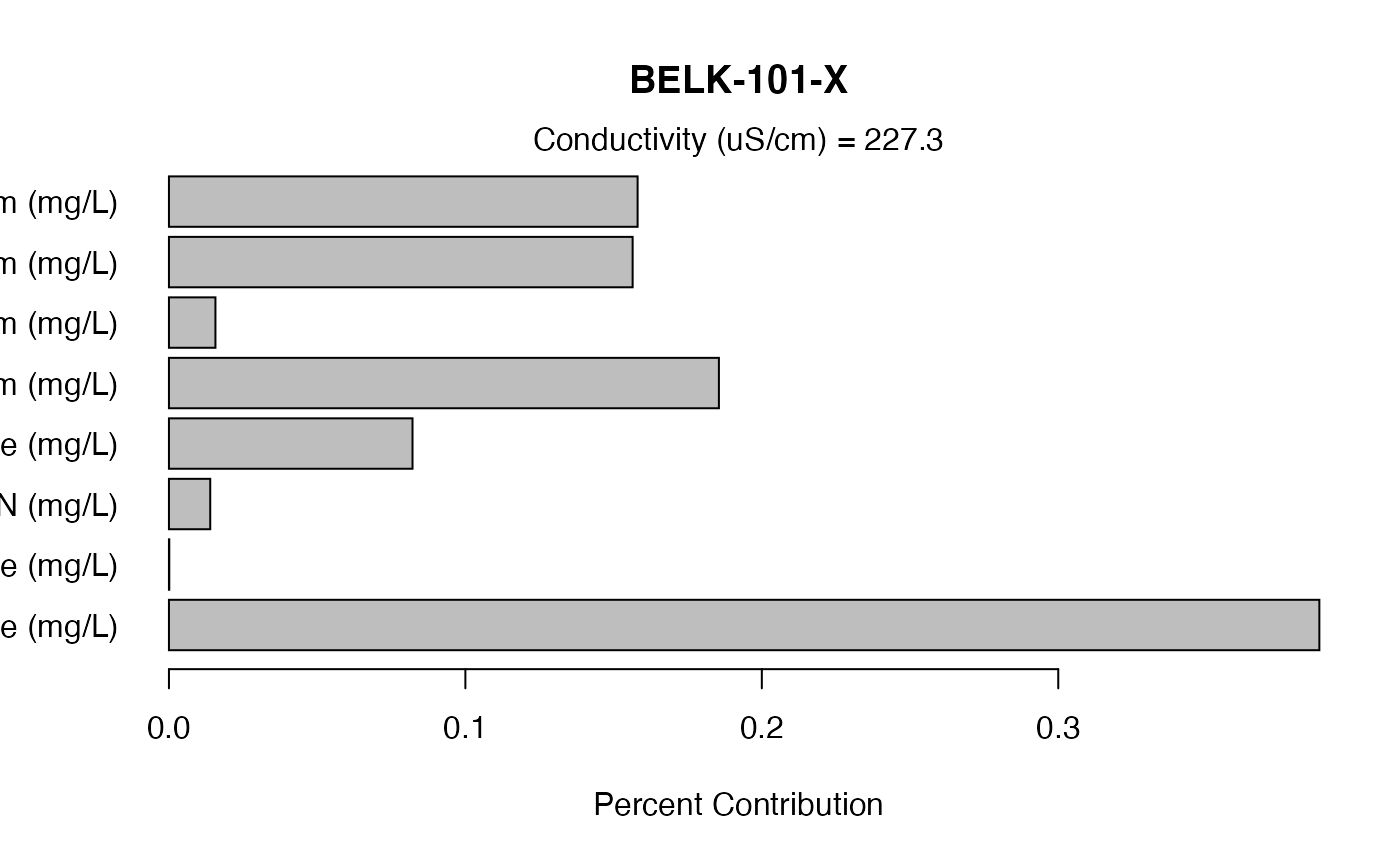
## Plot as a horizontal bar plot
# need to change margins to fit labels
#par(mai=c(1,2,1,1))
barplot(as.numeric(as.vector(data.plot[,myIons.Contrib])), names.arg=myIons, main=mySite, xlab="Percent Contribution"
, axes=TRUE, horiz=TRUE, las=1)
mtext(paste0("Conductivity (uS/cm) = ",round(data.plot[,"Cond.Total"],1)))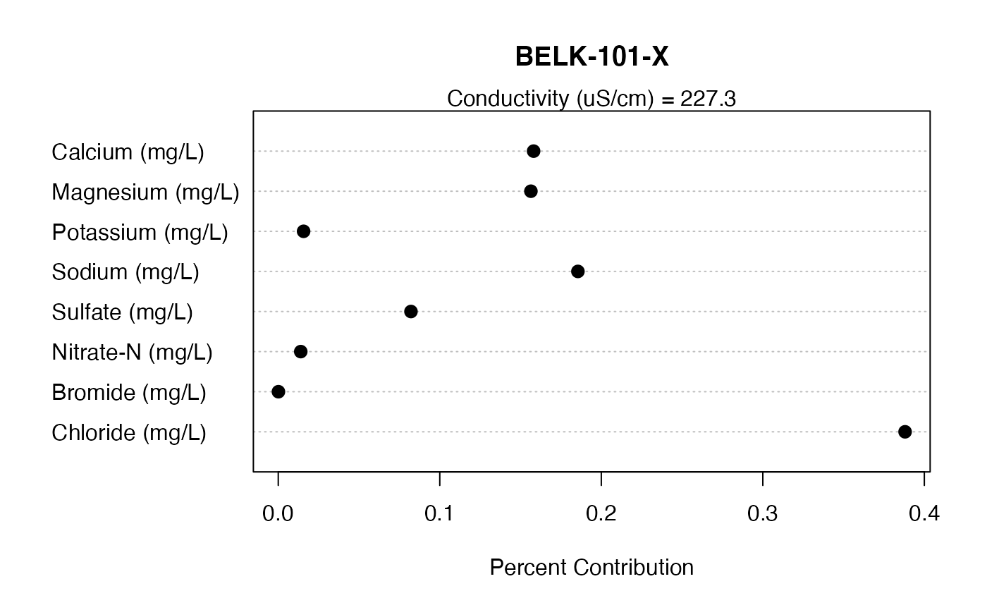
PHI
The PHIcalc() function calculates the MBSS Physical Habitat Index (PHI), Paul et al. 2003. The report is included in the /extdata folder of the library.
There are two versions of the calculation based on pre- and post-2000. The function determines the correct calculation based on the data provided.
The input is a data frame with column names matching the variables collected in the field along with SampleID, bioregion, and area (acres).
The function PHIcalc() requires no additional packages.
| StationID | SampleID | CollDate | Strata | PHICalcYear | Area_acres | Remote_020 | Shading_0100 | EpiSub_020 | BankStab_020 | AvgRipWid_m50max | InStrmHab_020 | InstrmWood_Num | RiffQual_020 | Embedd_0100 | Erosn_ExtR_075 | Erosn_ExtL_075 | Erosn_SevR_03 | Erosn_SevL_03 | RoadDist_m |
|---|---|---|---|---|---|---|---|---|---|---|---|---|---|---|---|---|---|---|---|
| AL-A-007-304-96 | NA | NA | Highland | 1994 | 8009.00 | 2 | 80 | 7 | 12 | 50 | NA | NA | NA | NA | NA | NA | NA | NA | NA |
| AL-A-020-228-95 | NA | NA | Highland | 1994 | 1335.26 | 17 | 90 | 1 | 5 | 50 | NA | NA | NA | NA | NA | NA | NA | NA | NA |
| AL-A-027-205-95 | NA | NA | Highland | 1994 | 2185.65 | 20 | 93 | 11 | 16 | 50 | NA | NA | NA | NA | NA | NA | NA | NA | NA |
| AL-A-027-209-95 | NA | NA | Highland | 1994 | 2428.11 | 19 | 97 | 11 | 15 | 50 | NA | NA | NA | NA | NA | NA | NA | NA | NA |
| AL-A-033-314-95 | NA | NA | Highland | 1994 | 9142.73 | 6 | 60 | 17 | 6 | 50 | NA | NA | NA | NA | NA | NA | NA | NA | NA |
| AL-A-054-320-96 | NA | NA | Highland | 1994 | 38907.00 | 1 | 60 | 5 | 16 | 0 | NA | NA | NA | NA | NA | NA | NA | NA | NA |
The function returns a dataframe of results that need to be saved (e.g., write.table()). The result table from the example data is shown below.
library(MBSStools)
# data
# MBSS.PHI = example dataset
myData <- MBSS.PHI
# calculate PHI
PHI <- PHIcalc(myData)
knitr::kable(head(PHI))| StationID | SampleID | CollDate | Strata | PHICalcYear | Area_acres | Remote_020 | Shading_0100 | EpiSub_020 | BankStab_020 | AvgRipWid_m50max | InStrmHab_020 | InstrmWood_Num | RiffQual_020 | Embedd_0100 | Erosn_ExtR_075 | Erosn_ExtL_075 | Erosn_SevR_03 | Erosn_SevL_03 | RoadDist_m | Erosn_SevR_02 | Erosn_SevL_02 | BANKSTAB1994 | BANKSTAB2000 | REMOTE1994 | REMOTE2000 | REMOTE | SHADING | EPI | BANKSTAB | RIPWID | INSTRHAB | WOOD | RIFFQUAL | EMBEDD | PHI.denom | PHI.sum | PHI |
|---|---|---|---|---|---|---|---|---|---|---|---|---|---|---|---|---|---|---|---|---|---|---|---|---|---|---|---|---|---|---|---|---|---|---|---|---|---|
| AL-A-007-304-96 | NA | NA | HIGHLAND | 1994 | 8009.00 | 2 | 80 | 7 | 12 | 50 | NA | NA | NA | NA | NA | NA | NA | NA | NA | NA | NA | 0.7097067 | NA | 0.10 | NA | 10 | 75.24754 | 38.888889 | 70.97067 | 100 | NA | NA | NA | NA | 5 | 295.1071 | 59.02142 |
| AL-A-020-228-95 | NA | NA | HIGHLAND | 1994 | 1335.26 | 17 | 90 | 1 | 5 | 50 | NA | NA | NA | NA | NA | NA | NA | NA | NA | NA | NA | 0.3560104 | NA | 0.85 | NA | 85 | 87.36514 | 5.555556 | 35.60104 | 100 | NA | NA | NA | NA | 5 | 313.5217 | 62.70435 |
| AL-A-027-205-95 | NA | NA | HIGHLAND | 1994 | 2185.65 | 20 | 93 | 11 | 16 | 50 | NA | NA | NA | NA | NA | NA | NA | NA | NA | NA | NA | 0.8640553 | NA | 1.00 | NA | 100 | 91.97549 | 61.111111 | 86.40553 | 100 | NA | NA | NA | NA | 5 | 439.4921 | 87.89843 |
| AL-A-027-209-95 | NA | NA | HIGHLAND | 1994 | 2428.11 | 19 | 97 | 11 | 15 | 50 | NA | NA | NA | NA | NA | NA | NA | NA | NA | NA | NA | 0.8274722 | NA | 0.95 | NA | 95 | 99.97552 | 61.111111 | 82.74722 | 100 | NA | NA | NA | NA | 5 | 438.8338 | 87.76677 |
| AL-A-033-314-95 | NA | NA | HIGHLAND | 1994 | 9142.73 | 6 | 60 | 17 | 6 | 50 | NA | NA | NA | NA | NA | NA | NA | NA | NA | NA | NA | 0.4174798 | NA | 0.30 | NA | 30 | 56.36867 | 94.444444 | 41.74798 | 100 | NA | NA | NA | NA | 5 | 322.5611 | 64.51222 |
| AL-A-054-320-96 | NA | NA | HIGHLAND | 1994 | 38907.00 | 1 | 60 | 5 | 16 | 0 | NA | NA | NA | NA | NA | NA | NA | NA | NA | NA | NA | 0.8640553 | NA | 0.05 | NA | 5 | 56.36867 | 27.777778 | 86.40553 | 0 | NA | NA | NA | NA | 5 | 175.5520 | 35.11040 |