Plot Oxythermal

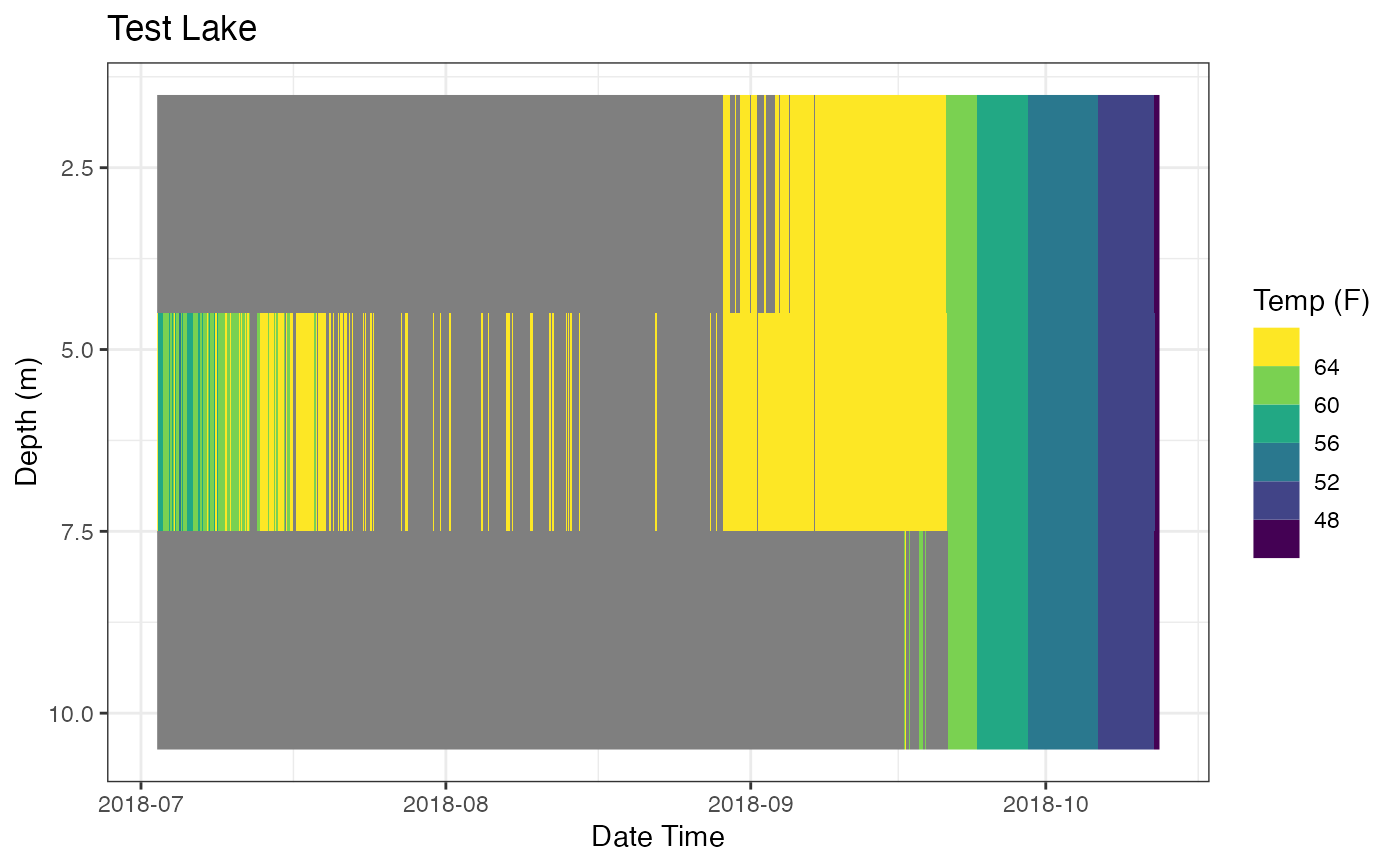
Generates a heat map of temperature from depth profile data. The data is filtered for temperature and dissolved oxygen levels prior to plotting.

plot_oxythermal(
  data,
  col_datetime,
  col_depth,
  col_temp,
  col_do,
  thresh_temp = 30,
  operator_temp = "<=",
  thresh_do = 3,
  operator_do = ">=",
  lab_datetime = NA,
  lab_depth = NA,
  lab_temp = NA,
  lab_title = NA,
  boo_interpolate = FALSE,
  boo_contours = FALSE
)

Arguments

data

data frame of site id (optional), data/time, depth , and measurement (e.g., temperature).

col_datetime

Column name, Date Time

col_depth

Column name, Depth

col_temp

Column name, Temperature

col_do

Column name, Dissolved Oxygen

thresh_temp

Threshold for temperature, Default = 30

operator_temp

Operator for temperature, Default is <= Valid values of >=, >, <=, <

thresh_do

Threshold for dissolved oxygen, Default is 3

operator_do

Operator for dissolved oxygen, Default is >= Valid values of >=, >, <=, <

lab_datetime

Plot label date time (x-axis), Default = col_datetime

lab_depth

Plot label for depth (y-axis), Default = col_depth

lab_temp

Plot label for temperatue (legend), Default = col_measure

lab_title

Plot title, Default = NA

boo_interpolate

Boolean as to use interpolate in geom_raster, Default = FALSE

boo_contours

Boolean to draw contours, Default = FALSE

Value

a ggplot object

Details

The heat map will show the acceptable habitat based on user inputs. Can be used with any parameters.

A plot is returned that can be saved with `ggsave(filename)`.

Labels (and title) are function input parameters. If they are not used the plot will not be modified.

The default theme is `theme_bw()`.

The plot is created with `ggplot2::geom_raster()`. Interpolation is possible with boo_interpolate (default is FALSE).

The returned object is a ggplot object so it can be further manipulated.

Examples

# Data (Test Lake)
data         <- laketest

# Column Names
col_datetime <- "Date.Time"
col_depth    <- "Depth"
col_temp     <- "temp_F"
col_do       <- "DO_conc"

# Data values
thresh_temp <- 68
operator_temp <- "<="
thresh_do <- 3
operator_do <- ">="

# Plot Labels
lab_datetime <- "Date Time"
lab_depth    <- "Depth (m)"
lab_temp     <- "Temp (F)"
lab_title    <- "Test Lake"

# Create Plot
p_ot <- plot_oxythermal(data = data
                        , col_datetime = col_datetime
                        , col_depth = col_depth
                        , col_temp = col_temp
                        , col_do = col_do
                        , thresh_temp = thresh_temp
                        , operator_temp= operator_temp
                        , thresh_do = thresh_do
                        , operator_do = operator_do
                        , lab_datetime = lab_datetime
                        , lab_depth = lab_depth
                        , lab_temp = lab_temp
                        , lab_title = lab_title)

# Print Plot
print(p_ot)


# Demo ability to tweak the plot
## move gridlines on top of plot
p_ot + ggplot2::theme(panel.ontop = TRUE
               , panel.background = ggplot2::element_rect(color = NA
                                                          , fill = NA))

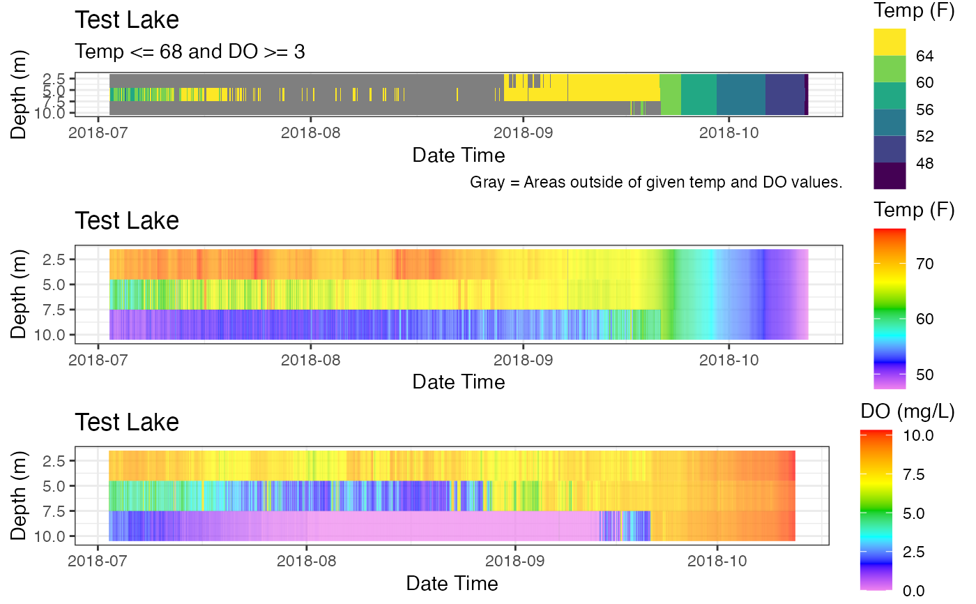
## Add subtitle and caption
myST <- paste0("Temp ", operator_temp, " ", thresh_temp
             , " and DO ", operator_do, " ", thresh_do)
p_ot <- p_ot +
  ggplot2::labs(subtitle = myST) +
  ggplot2::labs(caption = paste0("Gray = Areas outside of given"
                             , " temp and DO values."))

# save plot to temp directory
tempdir() # show the temp directory
#> [1] "/var/folders/24/8k48jl6d249_n_qfxwsl6xvm0000gn/T//Rtmp2bBrgJ"
ggplot2::ggsave(file.path(tempdir(), "TestLake_plotOxythermal.png")
                , plot = p_ot)
#> Saving 6.67 x 6.67 in image

# For Comparison, heatmaps of Temperature and DO

# heat map, Temp
p_hm_temp <- plot_heatmap(data = data
                     , col_datetime = col_datetime
                     , col_depth = col_depth
                     , col_measure = col_temp
                     , lab_datetime = lab_datetime
                     , lab_depth = lab_depth
                     , lab_measure = lab_temp
                     , lab_title = lab_title
                     , contours = FALSE)

# heat map, DO
p_hm_do <- plot_heatmap(data = data
                          , col_datetime = col_datetime
                          , col_depth = col_depth
                          , col_measure = col_do
                          , lab_datetime = lab_datetime
                          , lab_depth = lab_depth
                          , lab_measure = "DO (mg/L)"
                          , lab_title = lab_title
                          , contours = FALSE)

# Plot, Combine all 3
p_oxy3 <- gridExtra::grid.arrange(p_ot, p_hm_temp, p_hm_do)

p_oxy3
#> TableGrob (3 x 1) "arrange": 3 grobs
#>   z     cells    name           grob
#> 1 1 (1-1,1-1) arrange gtable[layout]
#> 2 2 (2-2,1-1) arrange gtable[layout]
#> 3 3 (3-3,1-1) arrange gtable[layout]

# save plot to temp directory
tempdir() # show the temp directory
#> [1] "/var/folders/24/8k48jl6d249_n_qfxwsl6xvm0000gn/T//Rtmp2bBrgJ"
ggplot2::ggsave(file.path(tempdir(), "TestLake_plotOxythermal_3.png")
                          , plot = p_oxy3)
#> Saving 6.67 x 6.67 in image