Plot Taxa Response Curve and Calculate Species Extirpation Concentrations
Source:R/taxon.response.sort.r
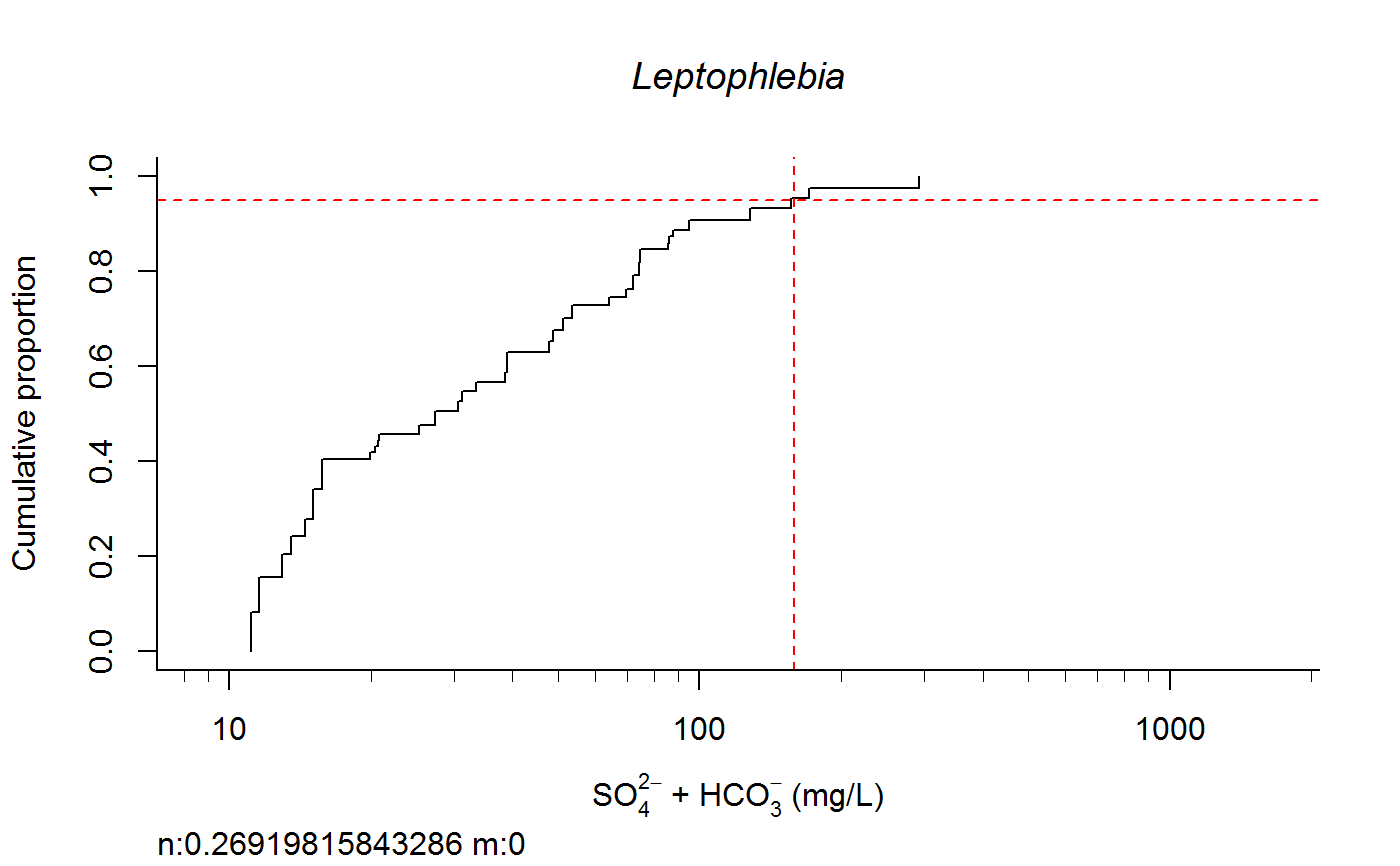
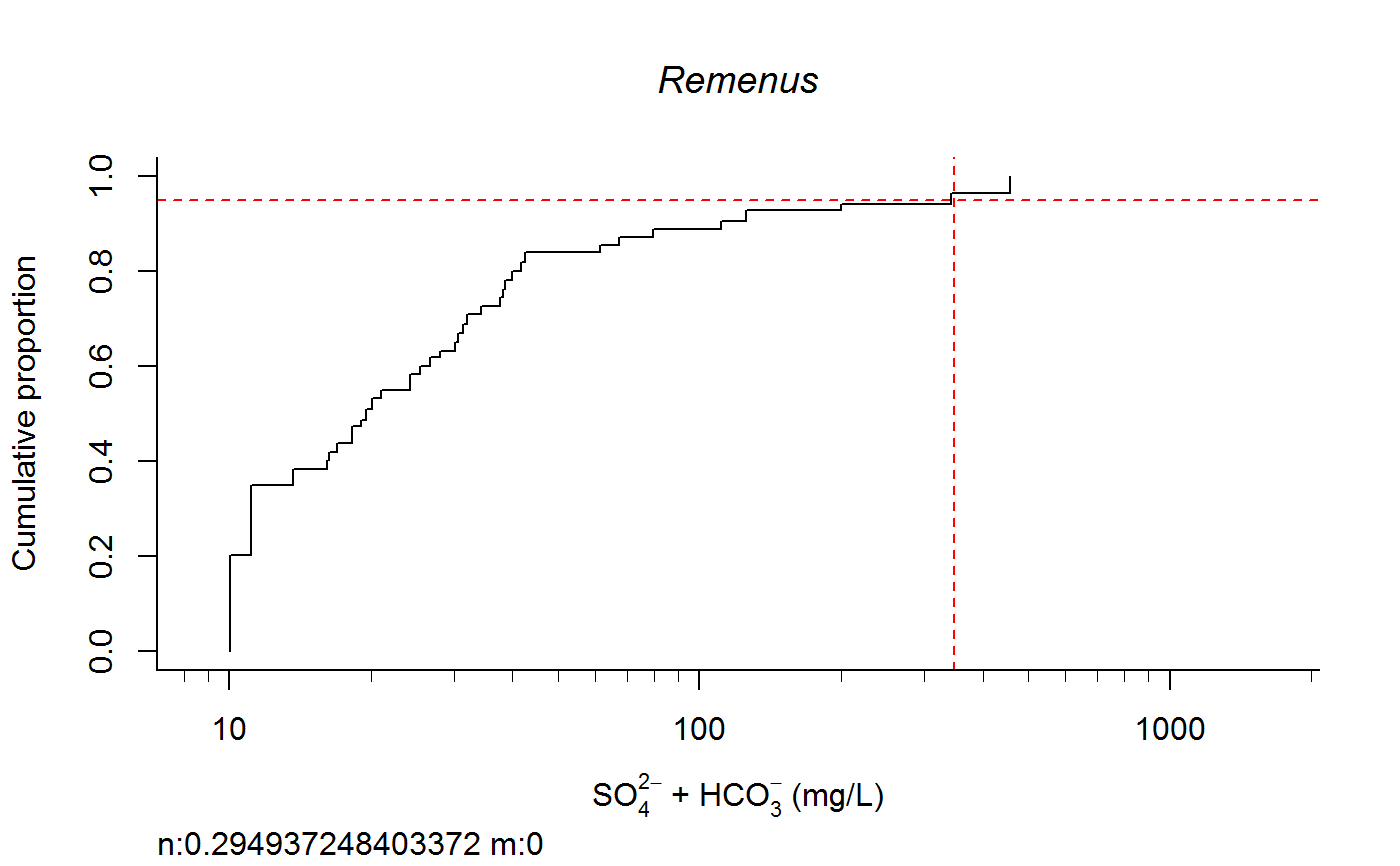
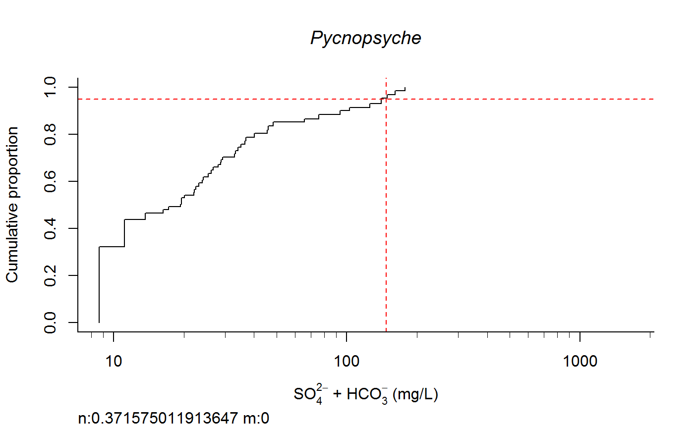
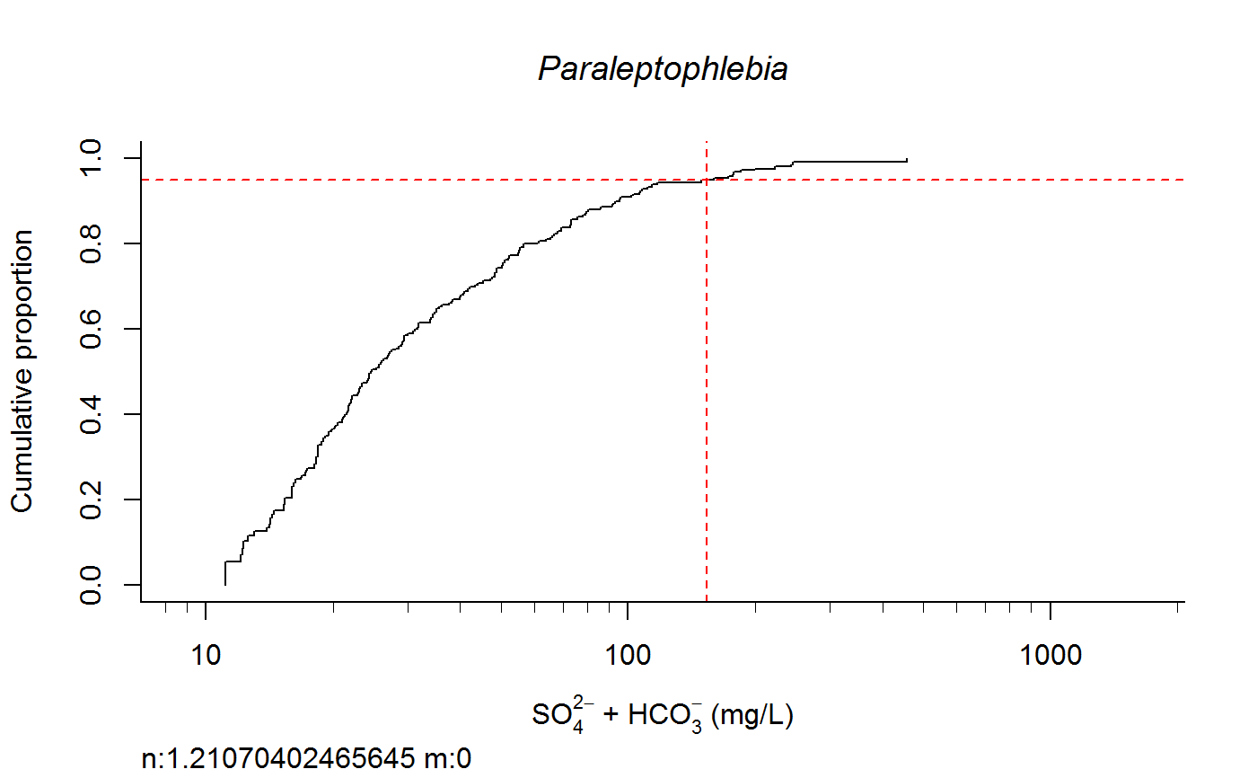
taxon.response.sort.RdThe output of this function to return 1.Weighted Average, 2. cdf_Abundance based, 3. cdf_ presence/absence based; 4. ecdf weighted, 5. cdf weight new; 6. Linear logistic regression, 7. quadratic logistic 8. GAM 5~7 using full data range; 9~11. repeat 6~8 but uses observed range for each single taxon; 12 Count. 13. Raw quantiles. Requires Hmisc for wtd.quantile() and Ecdf() and mgcv to gam().
taxon.response.sort(df1 = df1, xvar = "Conductivity", cutoff = 25,
  region = "all", mtype = 3, dense.N = 201, plot.pdf = F,
  xlabs = "Specific conductivity (uS/cm)", add.map = FALSE,
  GIS.cord = c("LONG_DD", "LAT_DD"), extirpation = NULL,
  maintext = "Macroinvertebrates response to specific conductivity",
  log.x = TRUE, rounder = 0, taus = c(0, 95, 100), nbin = 61,
  sort.vect = sort.vect, wd = getwd())
Arguments
| df1 | data frame |
|---|---|
| cutoff | a required minimum sample size for calculation |
| region | a subregion code to name the final output files |
| mtype | could be 1 to 3, indicating which regression model to use; default = 3. |
| dense.N | is the number of areas to cut into in the calculation of area under the curve |
| plot.pdf | to decide if we want species vs. env plots options "none", "pdf", "tiff" |
| add.map | to decide if a map should be added before plots. |
| maintext | title of the multiplots area |
| log.x | if xvar should be logtransformated |
| rounder | xvar rounder, default = 0 |
| taus | determine the output the percentile of env variable |
| nbin | number of bins for logits |
| sort.vect | when plot, sort the taxa list according to a vector called file called sort.vec |
| wd | Working directory for saving files. |
| xvar. | xvariable, could be column index or name |
Value
Output to the screen for each taxon as it is completed. CDF and GAM plots are saved to the specified directory in subfolders ("cdf" and "gam"). 1.Weighted Average, 2. cdf_Abundance based, 3. cdf_ presence/absence based; 4. ecdf weighted, 5. cdf weight new; 6. Linear logistic regression, 7. quadratic logistic 8. GAM 5~7 using full data range; 9~11. repeat 6~8 but uses observed range for each single taxon; 12 Count. 13. Raw quantiles
Examples
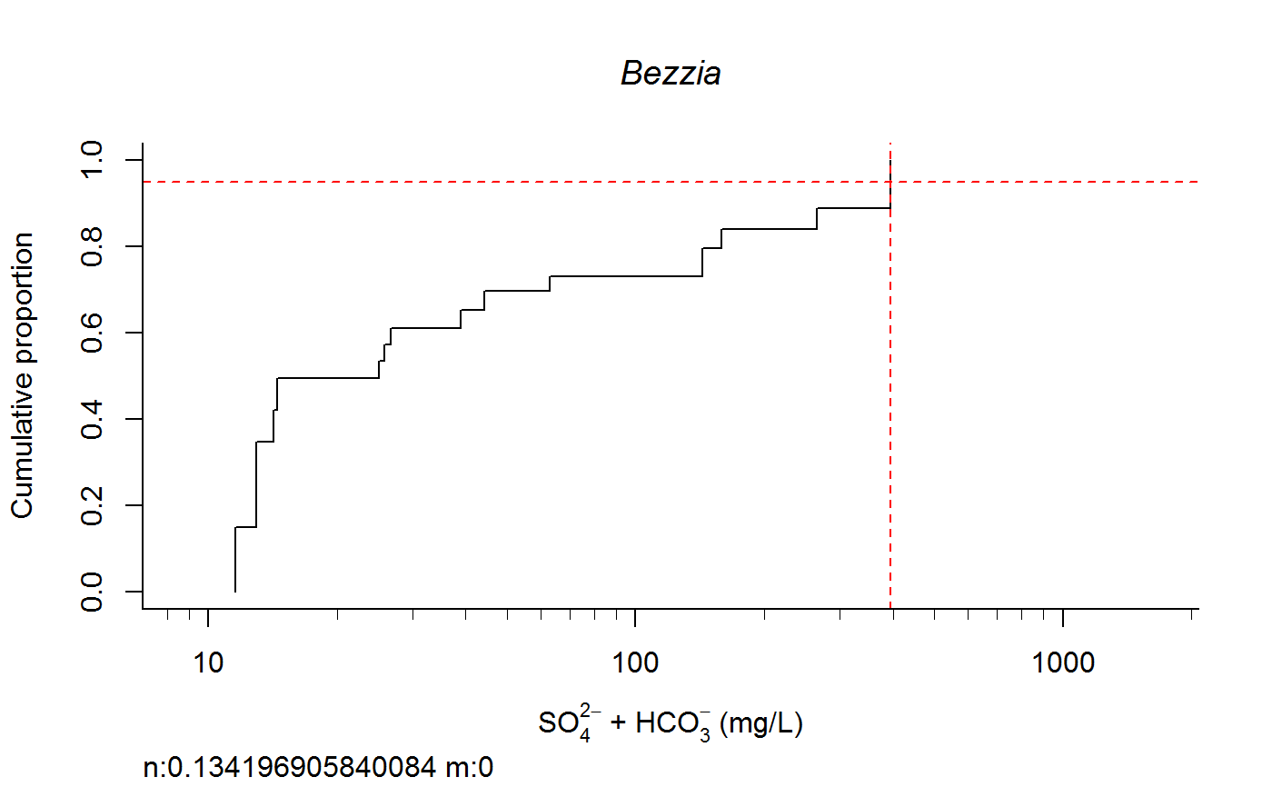
switch0 <- 1 ecolab <- ifelse (switch0 ==1, "eco69", "eco70") unitlab <- expression(paste("SO"[4]^{2-phantom()}," + HCO"[3]^{-phantom()}," (mg/L)")) full.results <- taxon.response.sort(df1 = df1, xvar = "lgSO4HCO3", cutoff = 25, region = ecolab , mtype = 3, dense.N = 201, plot.pdf = T, xlabs = unitlab, add.map = F, , maintext = "" , GIS.cord = c("Long_DD", "Lat_DD"), log.x = TRUE, rounder = 0, taus = c(0,95,100), nbin = 61, sort.vect = taxalist , wd=getwd())#> [1] 1#> [1] 2#> [1] 3#> [1] 4#> [1] 5#> [1] 6#> [1] 7#> [1] 8#> [1] 9#> [1] 10#> [1] 11#> [1] 12#> [1] 13#> [1] 14#> [1] 15#> [1] 16#> [1] 17#> [1] 18#> [1] 19#> [1] 20#> [1] 21#> [1] 22#> [1] 23#> [1] 24#> [1] 25#> [1] 26#> [1] 27#> [1] 28#> [1] 29#> [1] 30#> [1] 31#> [1] 32#> [1] 33#> [1] 34#> [1] 35#> [1] 36#> [1] 37#> [1] 38#> [1] 39#> [1] 40#> [1] 41#> [1] 42#> [1] 43#> [1] 44#> [1] 45#> [1] 46#> [1] 47#> [1] 48#> [1] 49#> [1] 50#> [1] 51#> [1] 52#> [1] 53#> [1] 54#> [1] 55#> [1] 56#> [1] 57#> [1] 58#> [1] 59#> [1] 60#> [1] 61#> [1] 62#> [1] 63#> [1] 64#> [1] 65#> [1] 66#> [1] 67#> [1] 68#> [1] 69#> [1] 70#> [1] 71#> [1] 72#> [1] 73#> [1] 74#> [1] 75#> [1] 76#> [1] 77#> [1] 78#> [1] 79#> [1] 80#> [1] 81#> [1] 82#> [1] 83#> [1] 84#> [1] 85#> [1] 86#> [1] 87#> [1] 88#> [1] 89#> [1] 90#> [1] 91#> [1] 92#> [1] 93#> [1] 94#> [1] 95#> [1] 96#> [1] 97#> [1] 98#> [1] 99#> [1] 100#> [1] 101#> [1] 102#> [1] 103#> [1] 104#> [1] 105#> [1] 106#> [1] 107#> [1] 108#> [1] 109#> [1] 110#> [1] 111#> [1] 112#> [1] 113#> [1] 114#> [1] 115#> [1] 116#> [1] 117#> [1] 118#> [1] 119#> [1] 120#> [1] 121#> [1] 122#> [1] 123#> [1] 124#> [1] 125#> [1] 126#> [1] 127#> [1] 128#> [1] 129#> [1] 130#> [1] 131#> [1] 132#> [1] 133#> [1] 134#> [1] 135#> [1] 136#> [1] 137#> [1] 138#> [1] 139#> [1] 140#> [1] 141#> [1] 142
